Solved Problem: Congestion Pricing and the Price Elasticity of Demand

Supports: Microeconomics and Economics, Chapter 6, and Essentials of Economics, Chapter 7, Section 7.5-7.7

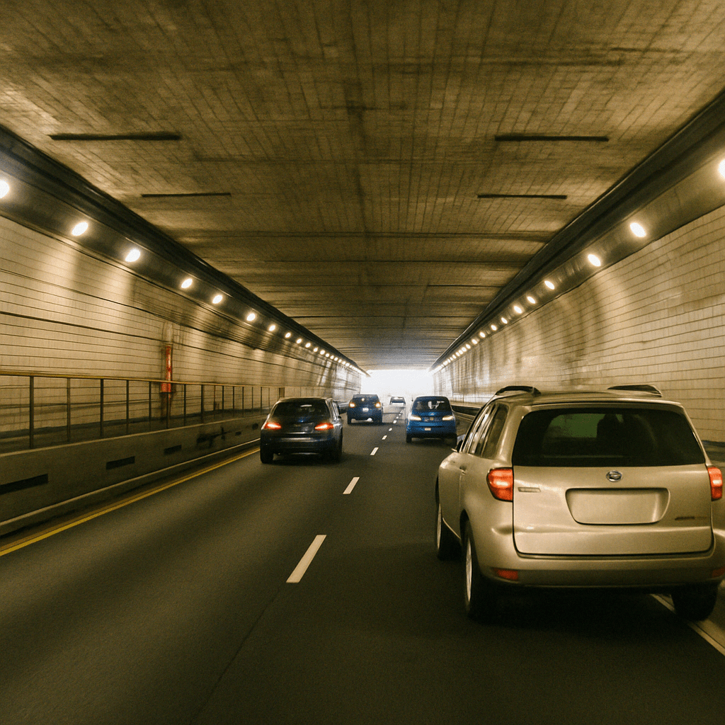
ChatGTP-4o image of cars in the Lincoln Tunnel, which connects New Jersey with midtown Manhattan.

In January 2025, New York City began enforcing congestion pricing in the borough of Manhattan south of 60th Street—the congestion relief zone. The Metropolitan Transportation Authority (MTA) in New York collects a toll from a vehicle entering that zone either automatically using the vehicle’s E-ZPass transponder or by reading the vehicle’s license plate and mailing a bill to the vehicle’s owner. Nobel Laureate William Vickrey of Columbia University first proposed congestion pricing in the 1950s as a way to deal with the negative externalities from traffic congestion. Congestion pricing acts as a Pigovian tax that internalizes the external costs drivers generate by using streets in congested areas. (We discuss Pigovian taxes in Microeconomics and Economics, Chapter 5, Section 5.3, and in Essentials of Economics, Chapter 4, Section 4.3.)

The New York City congestion toll is somewhat complex, varying according to the type of vehicle and how the vehicle enters the area in which the toll applies. The congestion toll fora car entering Manhattan through the Lincoln Tunnel on a weekday between 5 am and 9 pm is $6.00 on top of the existing toll of $16.06. In January 2025, the volume of cars driving through the Lincoln Tunnel declined by 8 percent during the weekday hours of 5 am to 9 pm. According to an article in Crain’s New York Business, the number of vehicles entering the congestion relief zone compared with the same month in the previous year declined by 8 percent in January, 12 percent in February, and 13 percent in March.

  1. From the information given, can we determine the price elasticity of demand for entering Manhattan by driving though the Lincoln Tunnel during weekdays from 5am to 9am? Briefly explain.
  2. Suppose someone makes the following claim: “Because the quantity of cars using the Lincoln Tunnel has declined by 8 percent, we know that the MTA must have collected less revenue from cars using the tunnel than before the congestion toll was imposed.” Briefly explain whether you agree.
  3. Is the pattern of increasing percentage declines in vehicle traffic in the congestion relief zone each month from January to March what we would expect? Be sure your answer refers to concepts related to the price elasticity of demand.

Step 1: Review the chapter material. This problem is about the price elasticity of demand, so you may want to review Chapter 6, Sections 6.1-6.4. 

Step 2: Answer part (a) by explaining whether from the information given we can determine the price elasticity of demand for entering Manhattan by driving through the Lincoln Tunnel. We do have sufficient information to determine the price elasticity, provided that nothing else that would affect the demand for driving through the Lincoln Tunnel changed during January. We’re told the percentage change in the quantity demand, so we need only to calculate the percentage change in the price to determine the price elasticity. The change in the price is the $6 congestion toll. The average of the price before and the price after the toll is imposed is ($16.06 + $22.06) = $19.06. Therefore, the percentage change in the price is ($6/$19.06) × 100 = 31.5 percent. The price elasticity of demand is equal to the percentage change in quantity dmanded divided by the percentage change in price: –6%/31.5% = –0.3. Because this value is less than 1 in absolute value, we can conclude that the demand for driving through the Lincoln Tunnel is price inelastic.

Step 3: Answer part (b) by explaining whether because the quantity of cars driving through the Lincoln Tunnel has declined the MTA must have collected less revenue from cars using the tunnel. As shown in Section 6.3 of the textbook, total revenue received will fall after a price increase only if demand is price elastic. In this case, demand is price inelastic, so the total revenue the MTA collects from cars using the Lincoln Tunnel will rise, not fall.

Step 3: Answer part (c) by explaining whether the pattern of increasing percentage declines in vehicle traffic in the congestion relief zone is one we would expect. In Section 6.2, we see that the passage of time is one of the determinants of the price elasticity of demand. The more time that passes, the more price elastic the demand for a product becomes. In other words, the longer the time that people have to adjust to the congestion toll—by, for instance, taking a bus rather than driving through the Lincoln Tunnel in a car—the more likely it is that people will decide not to drive into the congestion relief zone. So, it is not surprising that the number of vehicles entering the congestion relief zone declined by a greater percentage each month from January to March.

COVID-19 Update: Externalities During a Pandemic

Supports:  Hubbard/O’Brien, Chapter 5, Externalities, Environmental Policy, and Public Goods; Essentials of Economics Chapter 4, Market Efficiency & Market Failure

Apply the Concept: Should the Government Use Command-and-Control Policies to Deal with Epidemics?

Here’s the key point:   To deal with the negative externalities from an epidemic, a command-and-control policy may be more effective than a market-based policy.

The Externalities of Spring Break during the Coronavirus Epidemic

            When we think of negative externalities, we are typically thinking of externalities in production.   For example, a utility company that produces energy by burning coal causes a negative externality by emitting air pollution that imposes costs on people who may not be customers of that utility company.   During the coronavirus epidemic, some public health experts identified a significant negative externality in consumption.

            The coronavirus epidemic became widespread in the United States during March 2020—when many colleges were on spring break.  By mid-March several states including California, Washington state, and New York closed non-essential businesses such as hotels and restaurants, as well as parks and beaches. But many hotels, restaurants, and beaches in spring break destinations such as Florida remained open and   were packed with college students.  Many students realized that because of the crowds, they might catch the virus.

Why take the risk? There are two possible explanations.   First, many students likely agreed with an American University senior who was quoted in the Wall Street Journal as saying, “It’s a risk to be down here with crowds … [but] it’s my last spring break. I want to live it up as best I can.”  Second, some spring breakers were relying on early reports that people in their 20s who caught the virus would experience only mild symptoms or none at all.  But even young people with mild symptoms could spread the virus to others, including people older than 60 for whom the disease might be fatal.

            So, in March 2020 there was an externality in consumption from college students taking spring break beach vacations because people in large crowds spread the virus. In other words, the students’ marginal private benefit from being on the beach was greater than the marginal social benefit, taking into account that being on the beach might spread the virus.

            The following figure shows the market for spring break beach vacations. The price of a vacation includes transportation costs, renting a hotel room, meals, and any fees to use the beach.  Demand curve D1 is the market demand curve and represents the marginal private benefit to students from vacationing on a crowded beach during spring break.  But spring breakers don’t bear all the cost of potentially contracting the coronavirus by being on a crowded beach because the cost of their spreading the virus is borne by others. So, there is negative externality from vacationing on the beach equal to the vertical distance between D1, which represents the marginal private benefit, and D2, which represents the marginal social benefit, including the chance of spreading the virus by contracting it on a crowded beach.

Because of the externality, the actual number of people taking spring break beach vacations in March 2020, QMarket, was greater than the efficient number, QEfficient.  In Section 5.3 of the Hubbard and O’Brien textbook, we show that when there is an externality in production, a tax equal to the per unit cost of the externality will result in the efficient level of output because the tax causes firms to internalize the externality.  In a similar way, a tax on spring break beach vacations equal to the per unit cost of the externality would shift the marginal private benefit curve, D1, down to where it became the same as the marginal social benefit curve, D2.  By leading spring breakers to internalize the cost of the externality, the tax would cause the market quantity of beach vacations to decline to the efficient quantity, QEfficient.

In practice, however, imposing a tax on people taking a beach vacation would be difficult for two key reasons: (1) In March 2020, there were many aspects of the coronavirus, including how it spread and its fatality rate, that made calculating the value of the negative externality difficult, and  (2) collecting a tax on the many spring breakers crowded on beaches would have been administratively difficult. In the face of these factors, governors and mayors used the command-and-control approach in March of closing beaches, hotels, and restaurants rather than the market-based approach of levying a tax.

Sources: Arian Campo-Flores and Craig Karmin, “The Last Place to be Hit With Coronavirus Worries? Florida Beaches,” Wall Street Journal, March 21, 2020; Aimee Ortiz, “Man Who Said, ‘If I Get Corona, I Get Corona,’ Apologizes,” New York Times, March 24, 2020; and Ryan W. Miller, “’If I Get Corona, I Get Corona’: Coronavirus Pandemic Doesn’t Slow Spring Breakers’ Party,” usatoday.com, March 21, 2020.

Question 

According to news reports, some college students on spring break in March 2020 were unaware that partying on the beach put them at risk of contracting the coronavirus. Many also assumed that no one younger than 30 was at risk of becoming seriously ill from the virus, although, in fact, the virus did kill people in their 20s. Suppose that every student on spring break were completely informed about the risks of partying on the beach.  Using the figure above, briefly explain how each of the following would have been affected. Draw a graph to illustrate your answer.

a. the demand curve, D1

b. the demand curve, D2

c. QMarket

d. QEfficient

e. PMarket

f. PEfficient

g. Size of the deadweight loss

Instructors can access the answers to these questions by emailing Pearson at christopher.dejohn@pearson.com and stating your name, affiliation, school email address, course number.